World Cup 2026: How a Statistician Predicts Football Scores
Why the most likely score is not always the best pick.
The bad news first
Football predictions usually look more reasonable before kick-off than after the final whistle. Before the match, there are tables, odds, form curves, and arguments. Afterwards, there is an inside post, a VAR line, and the realization that predicting 2-1 was also just a very specific form of optimism.
The problem is not that we know nothing. Stronger teams win more often than weaker teams. Home advantage exists. Goals do not occur completely at random. The problem is that football has very few scoring events. A basketball game with 180 points can absorb a lot of small randomness. A football match with two or three goals cannot. If the first goal is somewhat accidental, it changes tactics, risk-taking, substitutions, and occasionally the emotional stability of the person who filled in the prediction sheet.
For a prediction game, this is annoying but interesting. We want to predict an exact score, even though the information we have about the match is rather fuzzy. That is why statistics is useful: it helps us manage our ignorance in an orderly way.
Why betting odds are a useful starting point
The obvious idea would be to build a model ourselves: team strength, squad quality, Elo ratings, expected goals, travel fatigue, weather, maybe even the emotional residue from the last press conference. This can be done. But it is easy to underestimate how much work it takes, how quickly relevant information can be missed, and how much noise additional variables can add to a model. Not every plausible predictor improves a forecast.
Betting odds are therefore attractive. They are not perfect truths, but they aggregate a lot of information: team strength, public news, market movements, injuries, expert judgement, and the assessments of many people who are financially motivated not to be wildly wrong. In the literature, odds are therefore often interpreted as forecasts. Forrest, Goddard, and Simmons (2005), for example, study football betting markets as forecasting tools. Kuypers (2000) discusses the efficiency of fixed-odds markets in English football. Classic work on football models and betting markets, such as Dixon and Coles (1997), does not treat odds as oracles, but does take them seriously as an information source.
This does not mean that bookmakers are altruistic prediction angels. Odds contain margins, can be distorted by demand, and are not designed to bring glory in private prediction leagues or questionable WhatsApp groups. But as a starting point, they are often better than a gut feeling that eventually says: “Portugal win 2-0, I can just see it.”
From odds to probabilities
Decimal odds can first be converted into implied probabilities by taking their reciprocal:1
\[ p_i^* = \frac{1}{q_i} \]
Odds of 2.00 therefore correspond roughly to a probability of 50 percent. Odds of 4.00 correspond to 25 percent. With three possible outcomes – home win, draw, away win – these raw probabilities usually add up to more than 100 percent. The difference is the bookmaker margin, often called the overround.
So we normalize:2
\[ p_i = \frac{p_i^*}{\sum_j p_j^*} \]
If the odds in Table 1 were offered for a match, they would imply the adjusted probabilities for the three basic outcomes shown in the table.
| Outcome | Odds | raw probability | normalized probability |
|---|---|---|---|
| Home win | 1.82 | 54.9 % | 52.8 % |
| Draw | 3.70 | 27.0 % | 26.0 % |
| Away win | 4.60 | 21.7 % | 20.9 % |
From this, we would roughly conclude: home win 53 percent, draw 26 percent, away win 21 percent. This is not yet a score prediction. It is only the broad direction.
The actual problem: We need an exact score
For a prediction game, “home win” is usually not enough. You need to enter 1-0, 2-1, or 3-2. Ideally, we would therefore use correct score odds, i.e. odds for exact results. If liquid and freely available odds existed for all possible scores, the procedure would be straightforward:
- Convert the odds for all scores into probabilities.
- Remove the bookmaker margin.
- Compute the expected point value for every possible prediction.
- Pick the prediction with the highest expected value.
In practice, this is harder. Correct-score odds are not always available, not always freely accessible, and sometimes not very liquid. A market on which hardly anyone trades is less helpful than a market with many bets. It therefore makes sense to use more widely available odds instead: 1X2 and, optionally, Over/Under 2.5.
1X2 means:
1: the home team wins,X: the match ends in a draw,2: the away team wins.
Over/Under 2.5 means:
Over 2.5: at least three goals are scored.Under 2.5: at most two goals are scored.
These odds do not directly tell us whether the match will end 1-0 or 2-1. But they say something about the relative team strengths and whether the match is expected to be low- or high-scoring.
From 1X2 to a score: the Poisson idea
If good correct-score odds are unavailable, we need a way to move from broad outcome odds to exact score probabilities. A long-standing standard model for football goals is the Poisson distribution. Dixon and Coles (1997) were already using Poisson-based models for football scores in the 1990s.
The basic idea is simple. For each team, we assume an expected number of goals:
- \(\lambda_{\text{home}}\): expected goals for the home team,
- \(\lambda_{\text{away}}\): expected goals for the away team.
Then the probability that a team scores \(k = 0, 1, 2, \dots\) goals is:
\[ P(Y = k) = \frac{\lambda^k e^{-\lambda}}{k!} \]
If we initially model the goals of the two teams as independent, the probability of a score \(i:j\) is the product:
\[ P(i:j) = P(Y_{\text{home}} = i) \cdot P(Y_{\text{away}} = j) \]
Of course, this is a simplification. Red cards, current scorelines, tactical adjustments, and tournament situations can create dependencies. For a private prediction game, however, the model is surprisingly useful: it turns a few market signals into a complete probability distribution over possible scores.
Siméon-Denis Poisson published a work on probabilities in criminal and civil judgements in 1837. So the original topic was not corner kicks, expected goals, or whether a 1-1 against Switzerland is a good result. Poisson (1837) was interested, among other things, in how to reason under uncertainty in legal judgements.
He would probably have been surprised to find his name in football prediction games. Then again, goals are rare count events, miscarriages of justice sometimes are too, and in both cases it helps not to confuse uncertainty with certainty.
How the calibration works
For the actual calculation, we do not simply guess which \(\lambda\) values might fit. Instead, \(\lambda_{\text{home}}\) and \(\lambda_{\text{away}}\) are chosen so that the resulting score grid matches the market probabilities as closely as possible. This is a small calibration problem: which two expected goal values produce a Poisson model whose home-win, draw, and away-win probabilities are closest to the probabilities implied by the odds?
Concretely:
- We choose preliminary values for \(\lambda_{\text{home}}\) and \(\lambda_{\text{away}}\), for example 1.4 and 1.1.
- From these, we compute all score probabilities from 0-0 up to, say, 7-7.
- We aggregate these score probabilities back into:
- home win,
- draw,
- away win.
- Optionally, we also compute the probability of
Over 2.5. - We then measure how far these model probabilities are from the market probabilities.
- Finally, an optimization procedure adjusts the two \(\lambda\) values until this distance is as small as possible.
One possible loss function is the sum of squared deviations:
\[ L(\lambda_{\text{home}}, \lambda_{\text{away}}) = \left(\hat p_{\text{home}} - p_{\text{home}}\right)^2 + \left(\hat p_{\text{draw}} - p_{\text{draw}}\right)^2 + \left(\hat p_{\text{away}} - p_{\text{away}}\right)^2. \]
Here, \(p_{\text{home}}\), \(p_{\text{draw}}\), and \(p_{\text{away}}\) are the market probabilities derived from the odds. The quantities \(\hat p_{\text{home}}\), \(\hat p_{\text{draw}}\), and \(\hat p_{\text{away}}\) are the corresponding probabilities implied by the Poisson score grid. If an Over/Under quote is included, another term is added that aligns the model probability of more than 2.5 goals with the market probability.
Technically, this is a small numerical optimization problem in two parameters. There is no useful closed-form expression for the two expected goal values here, because the win, draw, and Over/Under probabilities are made up of many individual Poisson probabilities. A derivative-free search method such as Nelder-Mead can be used (Nelder and Mead 1965). The logarithms of the \(\lambda\) values are optimized; after transforming them back with the exponential function, the expected goals are automatically positive.
Substantively, this is an attempt to reconstruct a plausible goal distribution from market information. The result is not a “true” score expectation, but a calibrated pair of expected goals that summarizes the available odds as well as possible.
Why not simply pick the most likely score?
Once we have a probability distribution over exact scores, a simple rule suggests itself: pick the most likely score. The calculation does not have to stop at 2-0 or 0-2. In practice, a larger score grid is considered, for example from 0-0 to 7-7. For presentation purposes, however, the most likely scores are usually enough. Suppose a model estimates, among other things, the values in Table 2.
| Score | Probability |
|---|---|
| 1-0 | 11.3 % |
| 1-1 | 11.1 % |
| 2-0 | 9.9 % |
| 2-1 | 9.8 % |
The most likely score is 1-0. So predict 1-0 and call it a day?
Not necessarily. In a prediction game, what matters is not only whether the exact prediction is the most likely one. What matters is how many points you expect to score on average. Under the standard Kicktipp rules, for example,3 you get:
- 4 points for the exact score,
- 3 points for the correct goal difference,
- 2 points for the correct tendency,
- 0 points otherwise.
This means that a prediction of 2-1 can be almost as good as, or even better than, 1-0, even if 1-0 is the more likely individual score. Why? Because 2-1 is compatible with many other home wins. If the match ends 3-2, the goal difference is correct; if it ends 2-0, at least the tendency is right. The best prediction is therefore the prediction with the highest expected value:
\[ E(\text{points} \mid t) = \sum_r P(r) \cdot \text{points}(t, r) \]
Here, \(t\) is the submitted prediction and \(r\) is a possible actual score. The expected value says: if this match were played many times under the same probabilities, how many points would this prediction yield on average?
This is the point at which one can confidently say in a prediction game: “I am not picking 2-1 because I believe it will be 2-1. I am picking 2-1 because it maximizes my expected points.” That sounds good. It still does not prevent somebody else from being ahead after predicting Spain 0-0 Cape Verde – not for modelling reasons, but because they once had a very nice holiday on those islands.
A real example: Ecuador against Germany
Let us take a real upcoming match: Ecuador against Germany in Group E. According to the FIFA match schedule, the match will take place on 25 June 2026 at New York New Jersey Stadium (FIFA 2026). When updating this post, a query of European bookmaker odds provided 1X2 and Over/Under 2.5 prices for the match (The Odds API 2026). Converted and adjusted for the 1X2 margin, they imply approximately:
- Ecuador win: 17.1 %
- Draw: 18.9 %
- Germany win: 64.0 %
- Over 2.5 goals: 61.5 %
The calibration gives approximately:
- \(\lambda_{\text{Ecuador}} = 1.01\)
- \(\lambda_{\text{Germany}} = 2.18\)
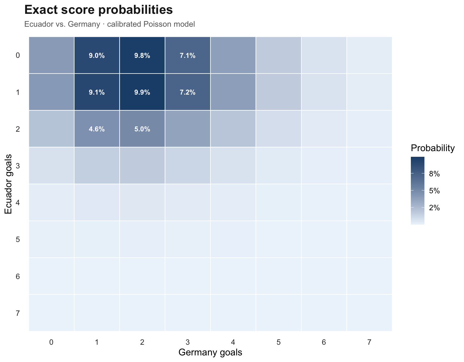
The model therefore expects about 1.01 Ecuadorian and 2.18 German goals on average. This produces a complete score grid. Figure 1 shows this grid as a heatmap; Table 3 shows only the most likely scores.
| Score | Probability |
|---|---|
| 1-2 | 9.9 % |
| 0-2 | 9.8 % |
| 1-1 | 9.1 % |
| 0-1 | 9.0 % |
| 1-3 | 7.2 % |
The most likely individual score is now 1-2. But we again compute the expected point value for every possible prediction in the score grid considered, not only for the five results in Table 3. Under the Kicktipp rules above, the top predictions are shown in Table 4.
| Prediction | expected points |
|---|---|
| 1-2 | 1.608 |
| 0-1 | 1.599 |
| 0-2 | 1.567 |
| 2-3 | 1.546 |
| 1-3 | 1.541 |
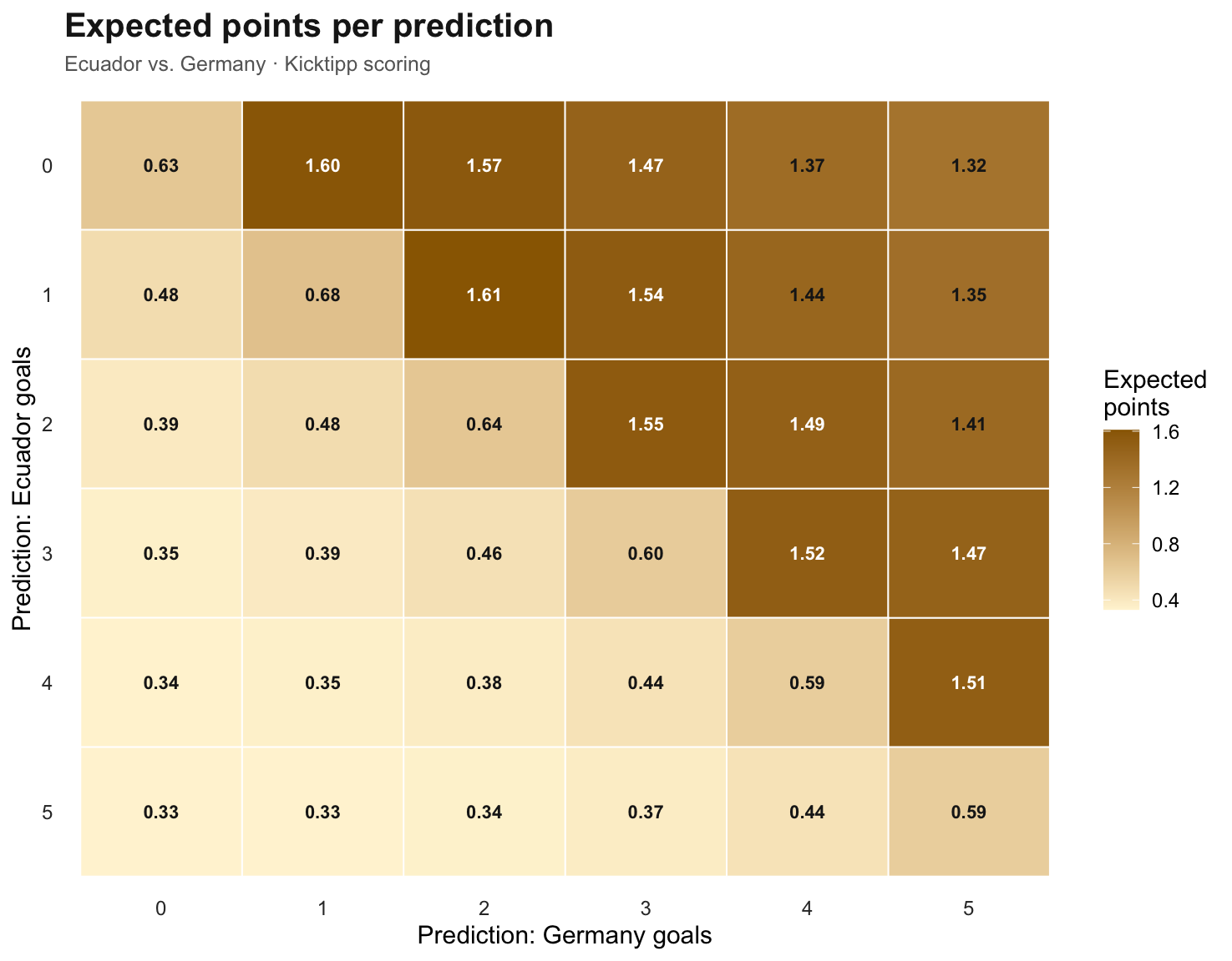
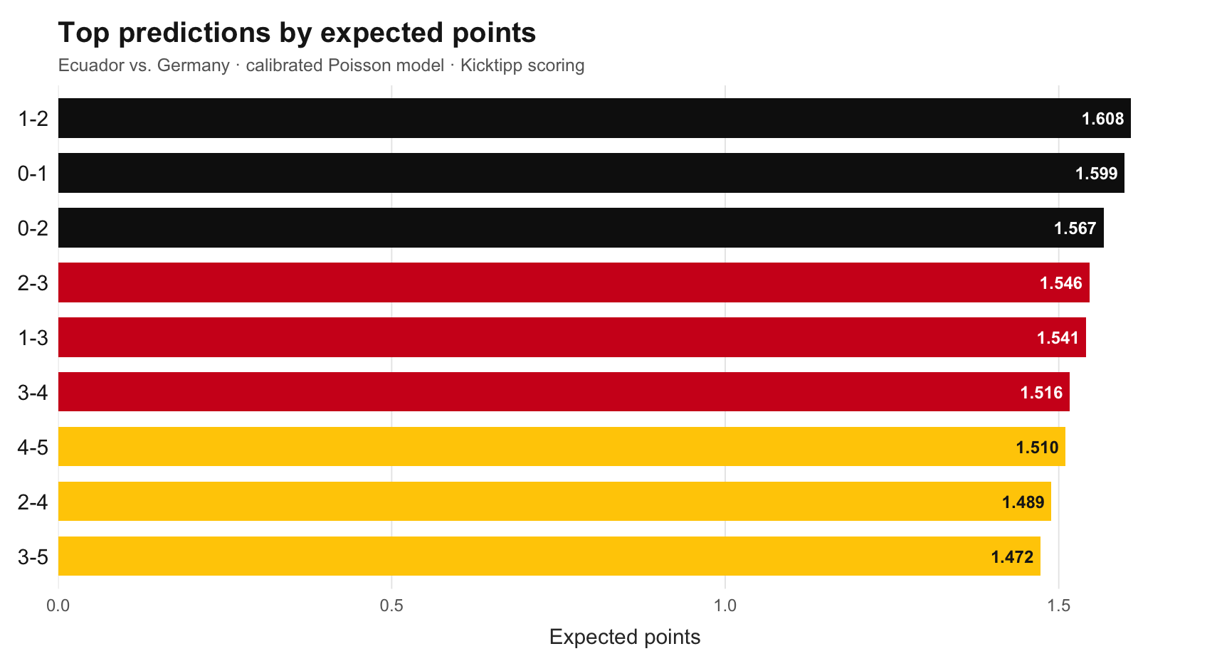
In this example, 1-2 wins. What is interesting, however, is how close 0-1 comes. Small changes in the odds or in the treatment of the Over/Under information can already be enough to change the ranking.
For now, the statistical pick would be: Ecuador 1-2 Germany. We will see whether it holds up. If the match ends 4-4, this was of course always a model for maximizing long-run expected points, not a short-term prophecy machine.
What could be improved
The model is deliberately pragmatic. For a prediction game, that is an advantage. On a Saturday morning, one does not necessarily want to write a dissertation on South American pressing resistance before entering a score. Still, there are possible extensions:
- Closing odds instead of early odds: Shortly before kick-off, odds usually contain more information than several days earlier.
- Team-specific models: Historical attacking strength, expected goals, injuries, or Elo ratings could be added.
- Correlation and low-score correction: Simple Poisson models can under- or overestimate certain low scores. Dixon-Coles models correct exactly such effects (Dixon and Coles 1997).
- Tournament context: In group-stage matches, a draw can be enough for both teams. At that point, football is no longer just a sport, but game theory with shin pads.
- Prediction-game strategy: If everyone else predicts favourite wins, it may be rational to take more risk depending on the leaderboard situation. But that is no longer pure expected-value maximization; it is tournament strategy.
Conclusion
Statistical prediction does not mean knowing the result. It means translating the available information into probabilities and then aligning the decision with the rules of the prediction game.
The key point is counterintuitive: the best prediction is not automatically the most likely score. The best prediction is the one with the highest expected point value. For that, we need a probability distribution over possible scores, a scoring system, and the willingness to say after a 0-0: “The model was right in expectation.”
That does not automatically win every prediction league. But it is statistically defensible.
References
Footnotes
Other odds formats can first be translated into decimal odds. American odds are expressed relative to a stake or profit of 100 units. Odds of +410 mean: a stake of 100 yields a profit of 410. As decimal odds, that is 5.10. Odds of -150 mean: you need to stake 150 to win 100. As decimal odds, that is about 1.67.↩︎
The resulting probabilities are not observed truths, but estimates derived from market prices. They depend, among other things, on bookmaker margins, market liquidity, the timing of the query, and possible biases in the betting market. Without an additional model for how the odds are generated, we cannot make classical claims about properties such as consistency or efficiency.↩︎
These rules can be customized, and one can spend a surprising amount of time debating which rules are best. If the rules differ, the method still works.↩︎