%%{init: {'theme': 'base', 'flowchart': {'htmlLabels': false}, 'themeVariables': { 'fontSize': '20px' }}}%%
flowchart LR
    U[User]
    UI[Internal chat interface]
    GW[Backend / Prompt gateway]
    CLF[Prompt classification<br/>classical ML + policy]
    DEC{Policy decision}
    LLM[LLM inference<br/>on-prem or EU-hosted]
    RET[Response to UI]
    LOG[(Audit log / monitoring)]
    REV[Human review]

    U --> UI --> GW --> CLF --> DEC
    DEC -->|Allow| LLM --> RET --> UI
    DEC -->|Warn / rewrite| GW
    DEC -->|Block / escalate| REV
    CLF --> LOG
    DEC --> LOG

    classDef user fill:#e6f4ff,stroke:#1d4ed8,color:#0f172a,stroke-width:2px,font-size:19px;
    classDef system fill:#eef2ff,stroke:#4f46e5,color:#111827,stroke-width:2px,font-size:19px;
    classDef decision fill:#fff7ed,stroke:#c2410c,color:#111827,stroke-width:2px,font-size:19px;
    classDef classifier fill:#dcfce7,stroke:#15803d,color:#052e16,stroke-width:4px,font-size:21px;
    classDef infra fill:#f5f3ff,stroke:#6d28d9,color:#111827,stroke-width:2px,font-size:19px;
    classDef review fill:#fee2e2,stroke:#b91c1c,color:#111827,stroke-width:2px,font-size:19px;

    class U user;
    class UI,GW,LLM,RET system;
    class DEC decision;
    class CLF classifier;
    class LOG infra;
    class REV review;
Prompt Classification with Classical Machine Learning
An embedding-based experiment using German Bundestag speeches
R
NLP
LLMs
Embeddings
Bundestag
AI-Act
I am currently working on the question of how prompts can be classified before execution to support governance decisions under the EU AI Act (European Union 2024).
The practical hurdle is straightforward: for AI-Act-style prompt risks, there is currently no broadly available, high-quality public gold-label dataset with fine-grained classes. So I start with a pragmatic but methodologically sound proxy: Bundestag speeches with known parliamentary group labels, collected via my R package bunddev (Bücker 2026).
This is also a useful stress test for the full setup: structured data collection, reproducible preprocessing, embedding features, multiclass evaluation, and explainability.
A concrete example: an employee enters the prompt “Summarize the latest supervisory board minutes regarding the planned acquisition” into the internal chat. A PII filter would see no issue — there is no personal data involved. But a content-level governance layer could flag the prompt as potentially confidential and trigger review or escalation.
That is exactly the layer this project targets: content-level prompt classification for governance/risk logic, not only PII detection. For narrower safeguards like PII detection, established filters already exist, for example NER-based detection with Microsoft Presidio.
Why companies build their own AI stacks
In practice, many companies already use AI productively, but often not through public default interfaces. Instead, they operate their own systems, either on-prem or EU-hosted. Common reasons include:
- Data protection and data residency
- Protection of trade secrets and intellectual property
- Compliance, audit, and accountability requirements
- Access control (roles, permissions, SSO)
- Integration with internal data and business workflows
- Cost control and provider/model flexibility
- Operational stability, monitoring, and incident handling
Architecturally, this often looks as shown in Figure 1: an internal chat interface receives input, backend services process prompts, and only then a model is called. Prompt classification acts as a governance layer between prompt intake and inference.
Requirements for an enterprise prompt classification system
In a production-grade, GDPR-compliant chatbot stack, a practical classifier should satisfy at least the following properties:
- Controllable decision logic: Risk decisions should not rely solely on a generative LLM; they should be grounded in stable, versioned procedures.
- Case-level transparency: If a prompt is blocked or flagged, the triggering signals should be explainable.
- Low latency: Pre-inference classification must not materially degrade UX.
- Determinism and reproducibility: Identical inputs under identical versions should produce consistent outcomes.
- Auditability: Scores, thresholds, policy/model versions, and timestamps should be logged.
- Fail-safe behavior: Uncertainty and partial outages need explicit fallbacks (for example, human review instead of silent allowance).
- Monitoring and drift management: Distribution shifts, class-wise errors, and threshold behavior should be tracked over time.
This requirement set favors fast, transparent classifiers plus an explicit policy layer rather than purely generative black-box decisions.
Dataset and filtering logic
Why this dataset?
For the actual AI-Act use case, public and cleanly labeled prompt-risk data is currently limited. With Bundestag speeches, we have a clearly defined classification target: the labels are parliamentary groups, and the task is to assign each speech to its correct group based on content. This yields a clean supervised multiclass problem.
Concretely, the dataset provides:
- clear class labels,
- semantic overlap across classes,
- enough variance for a realistic multiclass setup.
That mix makes it a useful methodological dry run.
| Parliamentary group | Number of speeches | Mean words | SD words | Median words | P25 words | P75 words | Min words | Max words | Seats (term 20) | Speeches per seat |
|---|---|---|---|---|---|---|---|---|---|---|
| AfD | 150 | 518.8 | 283.9 | 518.5 | 336.2 | 645.5 | 100 | 1,564 | 83 | 1.81 |
| Bündnis 90/Die Grünen | 173 | 604.8 | 309.8 | 591.0 | 422.0 | 752.0 | 101 | 2,170 | 118 | 1.47 |
| CDU/CSU | 279 | 656.6 | 405.2 | 623.0 | 441.5 | 767.0 | 102 | 3,290 | 197 | 1.42 |
| Die Linke | 83 | 438.5 | 244.2 | 407.0 | 304.0 | 495.0 | 107 | 1,482 | 39 | 2.13 |
| FDP | 157 | 624.2 | 324.6 | 603.0 | 443.0 | 748.0 | 101 | 2,210 | 92 | 1.71 |
| SPD | 261 | 646.6 | 306.1 | 636.0 | 447.0 | 773.0 | 100 | 2,673 | 206 | 1.27 |
Table 1 shows the final class distribution, seat counts as a structural context factor, and relative activity via “Speeches per seat”. Spread measures for speech length are included as well. Part of the variation in speech counts is expected: larger groups have more potential speakers and typically produce more contributions (Federal Returning Officer of Germany 2021). The observation window is identical for all classes (Nov 13, 2024 to Mar 18, 2025). The classes are clearly imbalanced. This is typical not only for parliamentary data but likely also for future prompt-risk classes. That is exactly why this setup is useful as a fairness and robustness test.
| Processing step | Number of speeches | Excluded vs previous step |
|---|---|---|
| Raw input | 1,588 | 0 |
| Known group + text available | 1,339 | 249 |
| Target groups only (AfD, CDU/CSU, Greens, Linke, FDP, SPD) | 1,248 | 91 |
| Minimum length: 100 words | 1,133 | 115 |
| Duplicates removed | 1,103 | 30 |
The filtering logic in Table 2 is important for interpreting downstream results:
- Keep only speeches with usable text and known parliamentary group.
- Restrict to the target classes.
- Remove very short speeches (under 100 words) to avoid extremely thin signals.
- Remove duplicates.
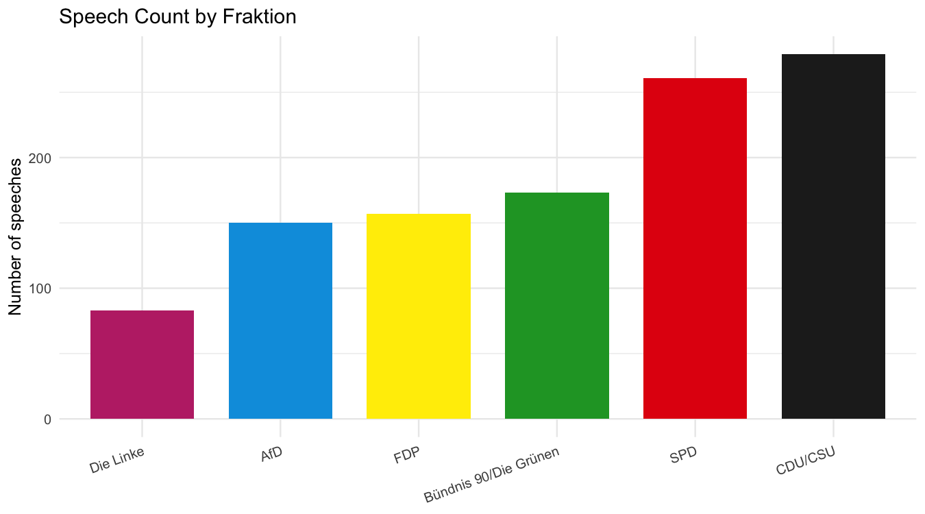
Figure 2 makes class imbalance visible.
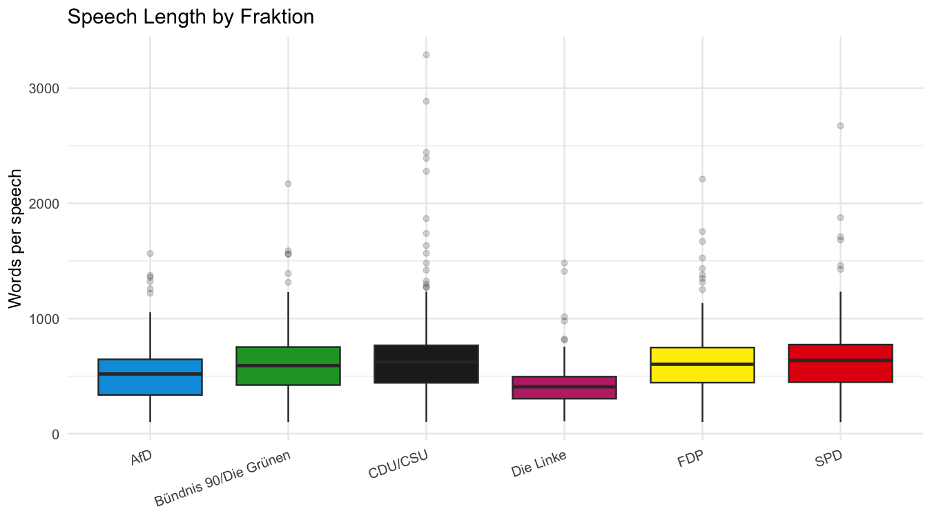
Figure 3 shows differences in speech length across classes. This matters for transfer to prompt use cases: user prompts are typically much shorter than parliamentary speeches. So the results are methodologically informative, but not directly transferable 1:1 to short prompt texts.
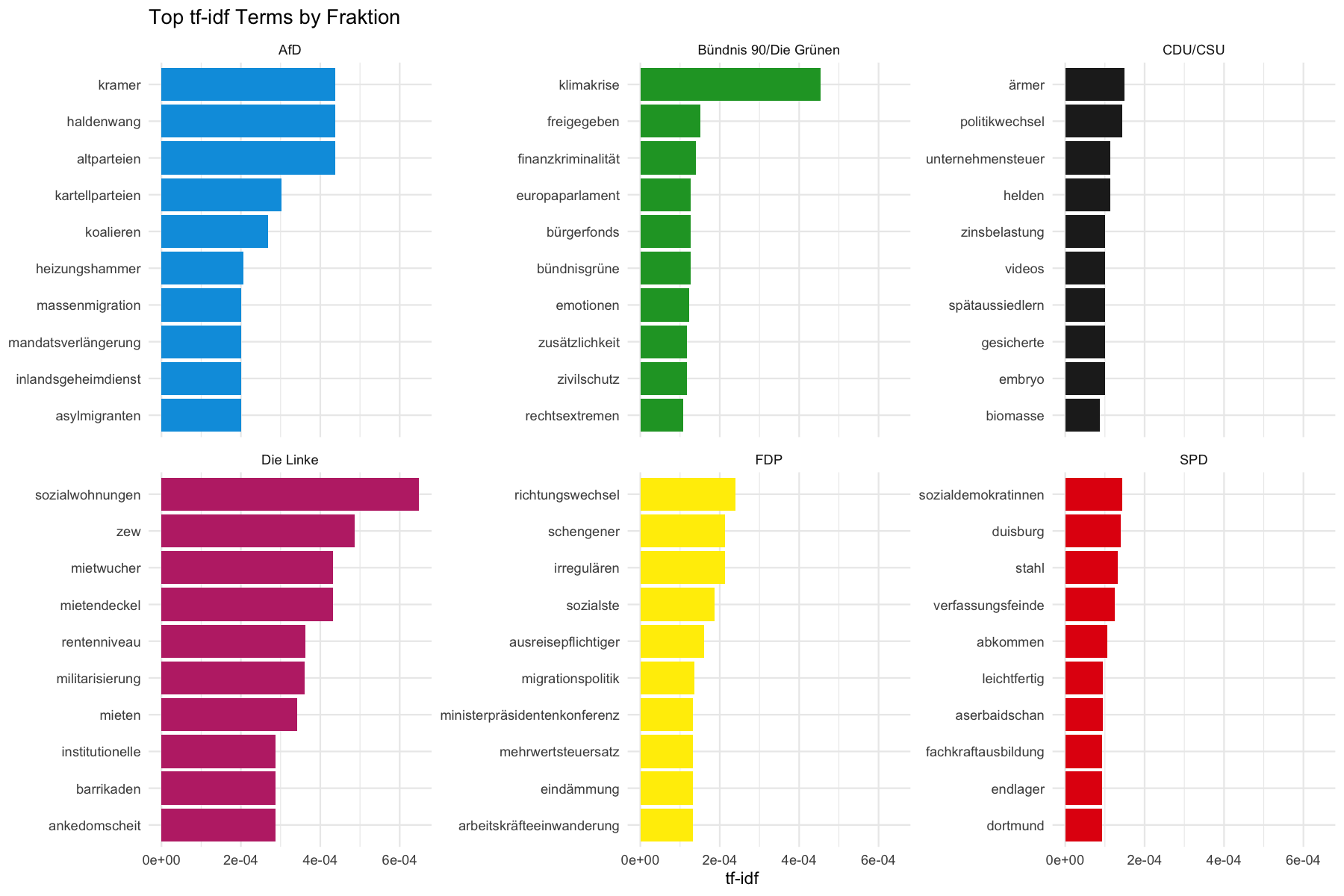
Figure 4 already indicates, before model training, that group-specific language patterns exist while thematic overlap is substantial. Short reminder: tf-idf upweights terms that are frequent in one subset but comparatively rare in the overall corpus. Formally: \[ \mathrm{tfidf}(t,d) = \mathrm{tf}(t,d) \cdot \log\!\left(\frac{N}{\mathrm{df}(t)}\right) \] with term \(t\), document/subcorpus \(d\), total number of documents \(N\), and document frequency \(\mathrm{df}(t)\). Here, \(\mathrm{tf}(t,d)\) is the relative frequency of term \(t\) in \(d\), while \(\mathrm{df}(t)\) counts in how many documents the term appears at all. This downweights very generic terms and highlights more characteristic ones.
In Figure 4, illustrative examples include terms such as “Verfassungsfeinde”, “Fachkraftausbildung”, “Brandmauern”, “Mietendeckel”, or “Rezession”. At the same time, overlap across parties remains visible in policy areas like migration, economy, or security.
Methodology
Feature representation
The baseline representation is a speech embedding: each full speech is encoded as a single vector. Embeddings were generated via Azure OpenAI using text-embedding-3-large.
In addition, chunk-based variants were evaluated:
- fixed segmentation, e.g. 150 words,
- smaller chunks (120 words) with 30-word overlap,
- pooling back to speech level (for example, averaging class probabilities).
Why compare these variants?
- Speech embeddings are efficient and easy to operate.
- Chunking can capture local class cues better.
- Chunking also improves local explainability by exposing concrete evidence passages.
Model families and selection criteria
For baseline selection, I intentionally started with multinomial logistic regression and a linear Support Vector Machine (SVM). The rationale is both practical and methodological:
- both models are well-suited to high-dimensional embedding features,
- both train and infer quickly,
- both provide robust reference lines before moving to more complex ensembles,
- both are more transparent than many heavyweight end-to-end alternatives.
Multinomial log-reg is a clean probabilistic reference: calibration is straightforward, interpretation is accessible, and it is an effective first reality check for linear separability.
Linear SVM is often strong in this regime because it optimizes class separation via the margin and tends to generalize robustly under noisy, overlapping classes (Cortes and Vapnik 1995).
NoteSupport Vector Machines
I have been fascinated by support vector machines since university. The combination of an elegant optimization problem (maximum margin under constraints), geometric intuition, and generalization perspective through VC ideas (Vapnik and Chervonenkis 1971) remains compelling to me in both theory and practice.
For intuition, Figure 5 shows the classic margin illustration.
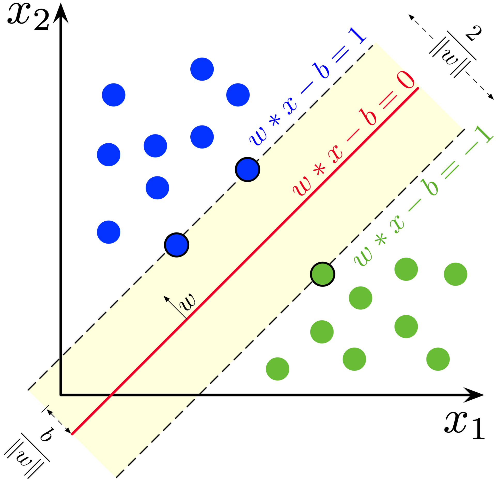
In simple terms, SVM first seeks a separating function that best distinguishes classes. For linear SVM, this is a hyperplane in feature space; nonlinear variants move separation into a suitable feature space.
The core ideas are:
- Maximum margin: instead of just any separating hyperplane, SVM seeks the one with largest distance to nearest points.
- Kernel trick: nonlinear structure can be modeled via implicit feature maps without explicitly computing high-dimensional coordinates.
- Generalization bias: large margins act like regularization and can reduce overfitting.
The evaluated model families were:
- Linear SVM on speech embeddings
- Multinomial logistic regression on speech embeddings
- Chunk-based logistic models with alternative pooling strategies
- Stacking/calibration as performance-oriented combinations of multiple signals
The key question was not only “which model has the best point estimate”, but: which approach remains robust, transparent, and production-practical at similar performance?
Resampling and evaluation strategy
The central evaluation axis is grouped speaker cross-validation (grouped CV). Speaker groups are separated between training and validation folds.
Why this matters:
- Without grouping, models can confuse speaker-specific style with class signal.
- That yields over-optimistic validation scores.
- Grouped CV is therefore a stricter test of generalization across speakers.
A separate test split is reported in addition. However, model selection prioritizes grouped-CV outcomes because they better reflect the target robustness requirement.
Metrics for an imbalanced multiclass setup
This is an imbalanced multiclass problem. Common options include:
- Accuracy: intuitive, but can be biased toward large classes under imbalance.
- Macro-F1: equally weights classes and balances precision/recall per class.
- Balanced Accuracy: mean recall across classes, robust under class imbalance.
- (optional) Weighted F1: accounts for class prevalence, but may underemphasize minority classes.
In this project, I use Macro-F1 as primary metric, Balanced Accuracy as secondary, and Accuracy as supplementary. This ordering is, in my view, the fairest for this setup.
Results
Reading guide: first, selected 6-class model performance; second, model comparison on the primary metric; third, a fair 2-class excursus; finally, confusion-matrix error patterns.
The selected model is a calibrated stacking ensemble that combines signals from SVM and logistic regression and uses class-specific thresholds for final assignment. It reaches grouped-CV Macro-F1 0.5622, Balanced Accuracy 0.7367, and Accuracy 0.5616. On the separate test split, the scores are Macro-F1 0.6090, Balanced Accuracy 0.7568, and Accuracy 0.6009.
In practical terms, this means roughly 56 out of 100 predictions are correct in grouped CV and roughly 60 out of 100 on the test split. For context, random guessing over six classes would be about 16.7%. A fairer comparison uses chance-normalized lift: 0.4740 in grouped CV and 0.5211 on test split.
| Model | Accuracy | Balanced Accuracy | Macro-F1 |
|---|---|---|---|
| Stack calibrated + threshold | 0.5616 | 0.7367 | 0.5622 |
| Stack uncalibrated | 0.5486 | 0.7410 | 0.5434 |
| Speech SVM | 0.5465 | 0.7405 | 0.5452 |
| Speech LogReg (weighted) | 0.5402 | 0.7306 | 0.5407 |
Table 3 complements the chart and makes metric-level comparisons easier to read.
Excursus: 2-class test and fair comparison
As a methodological side test, I also evaluated a binary setup: Government (SPD, Greens, FDP) vs Opposition (CDU/CSU, AfD, Die Linke). This uses the same embeddings as the main setup; only label mapping changes (6 classes vs 2 classes).
A fair comparison is essential: raw Accuracy is not directly comparable between 6-class and 2-class settings. So I compare Accuracy, Balanced Accuracy, and F1, and add chance-normalized lift: \[ \text{Lift} = \frac{\text{Accuracy} - \text{Chance}}{1 - \text{Chance}} \] with chance baseline \(1/6\) for the 6-class setup and \(1/2\) for the 2-class setup.
| Setting | Model | Accuracy | Chance baseline | Chance-normalized lift | Balanced Accuracy | F1 |
|---|---|---|---|---|---|---|
| 6 classes | Stack calibrated + threshold | 0.5616 | 0.1667 | 0.4740 | 0.7367 | 0.5622 |
| 2 classes | Linear SVM | 0.7487 | 0.5000 | 0.4974 | 0.7419 | 0.7153 |
Table 4 shows the expected effect: the 2-class problem is easier in absolute terms (higher Accuracy/Balanced Accuracy/F1). After chance normalization, both settings are notably closer together (6-class lift: 0.4740; 2-class lift: 0.4974). This suggests that embeddings do contain substantial signal, while the core difficulty lies in finer separation within the 6-class setup.
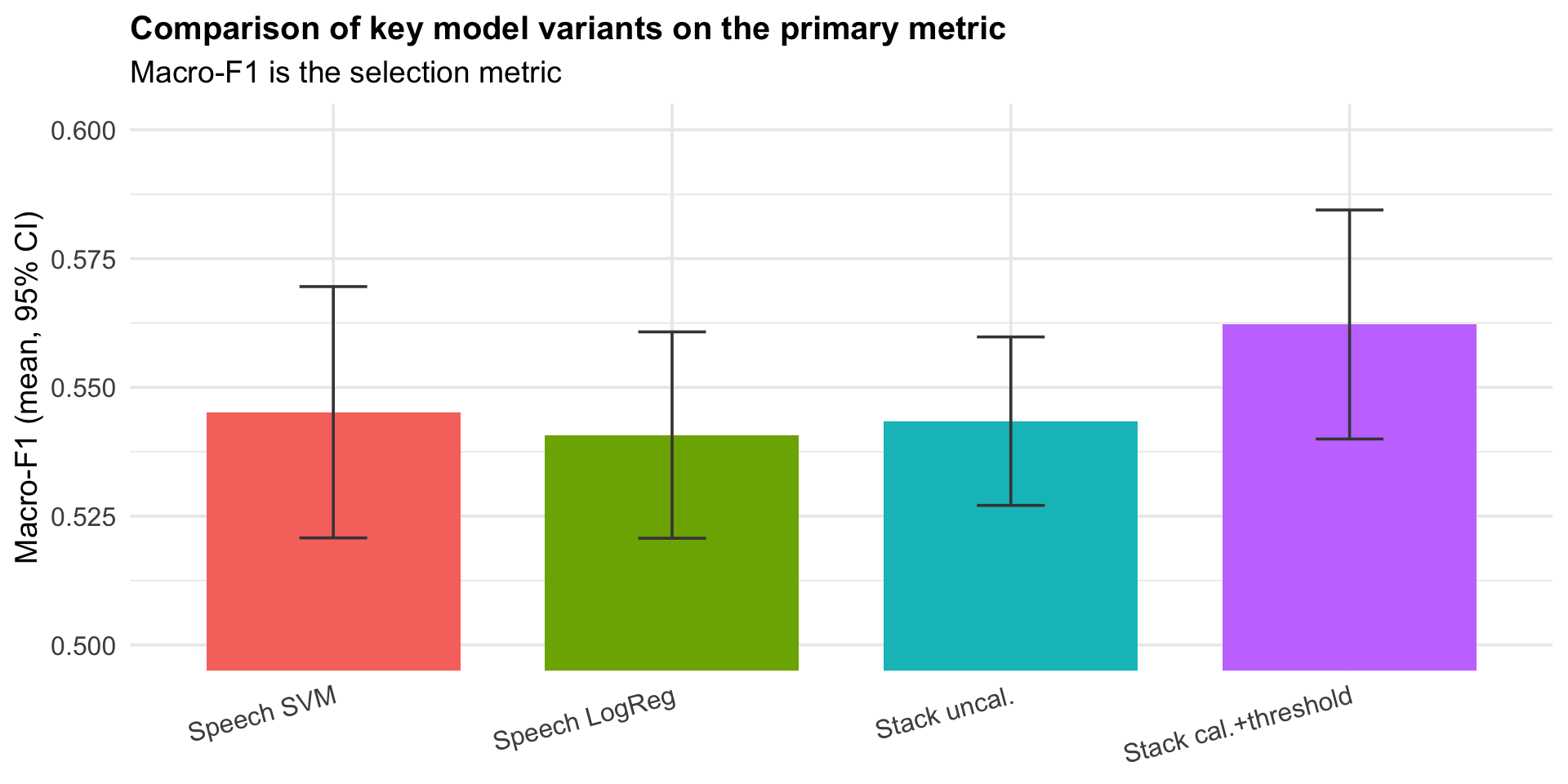
Additional metrics (Accuracy and Balanced Accuracy) are shown in Table 3.
Detailed interpretation of results
The selected stack model was chosen through a multi-step decision, not a single score. Primary criterion was grouped-CV Macro-F1, complemented by Balanced Accuracy (class fairness) and stability on the separate test split. On that combination, the calibrated stacking ensemble performs best while remaining robust enough to serve as a strong reference.
At the same time, Table 3 and Figure 6 show that the gap to linear speech-level SVM is limited. That matters operationally: if simplicity, maintainability, and explainability are weighted higher than the last bit of performance, linear SVM remains a very strong production-first choice.
Substantively, performance is solid but below an intuitive expectation: one might expect party assignment from content and vocabulary to be easier. The results indicate a structurally harder signal:
- Many speeches discuss similar policy domains.
- Embeddings place semantically similar contexts close together.
- Group-specific differences often live in finer rhetorical nuance rather than coarse topical clusters.
Those nuances are not always fully separable with standard embeddings alone.
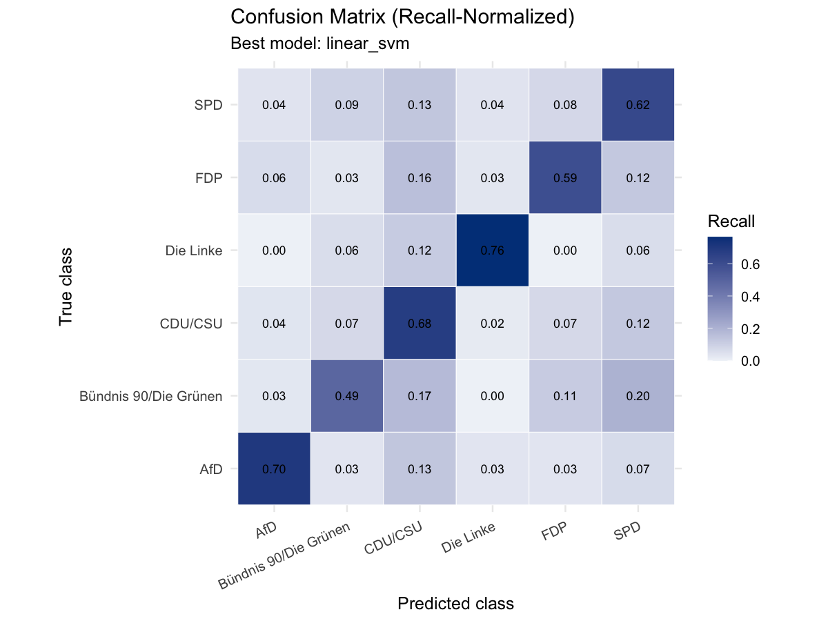
The confusion matrix in Figure 7 also shows that errors are not random; they concentrate between content-near parties. This points to plausible semantic overlap patterns rather than pure artifact-driven overfitting.
Concretely, the matrix can be read as “expected but asymmetric overlap”:
- Greens are relatively often predicted as SPD (0.20), while SPD -> Greens is notably smaller (0.09).
- Greens -> CDU/CSU is 0.17, which is indeed non-trivial; the reverse CDU/CSU -> Greens is 0.07.
- CDU/CSU vs SPD confusion is comparatively symmetric (SPD -> CDU/CSU: 0.13, CDU/CSU -> SPD: 0.12).
- AfD is more often shifted toward CDU/CSU (0.13) than to other classes, suggesting topic proximity in some debate areas.
In short: the model primarily confuses politically close parties — a substantively plausible pattern, not an artifact.
For prompt-risk classification, this is a key takeaway: when classes are semantically close, systematic boundary cases are expected and should be addressed via review/escalation design.
Explainability
Explainability is not optional in this context; it is a core requirement. A risk decision without justification is hard to defend operationally and regulatorily.
Conceptually, two levels are useful (Ribeiro, Singh, and Guestrin 2016; Lundberg and Lee 2017; Doshi-Velez and Kim 2017; Bücker et al. 2021):
- Local: Why was this specific instance classified this way?
- Global: Which recurring patterns does the model use per class?
This split can be read as a simplified explanation pyramid where local and global views are combined systematically (Bücker et al. 2021).
In this project, I use chunk-level evidence plus term-level aggregations.
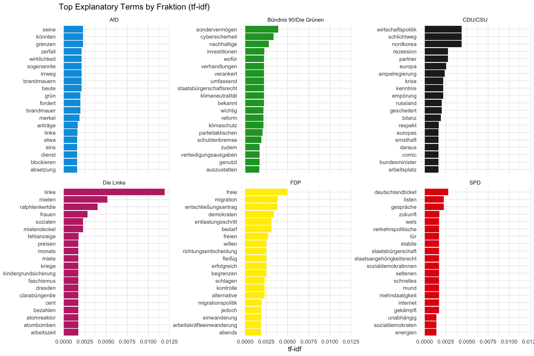
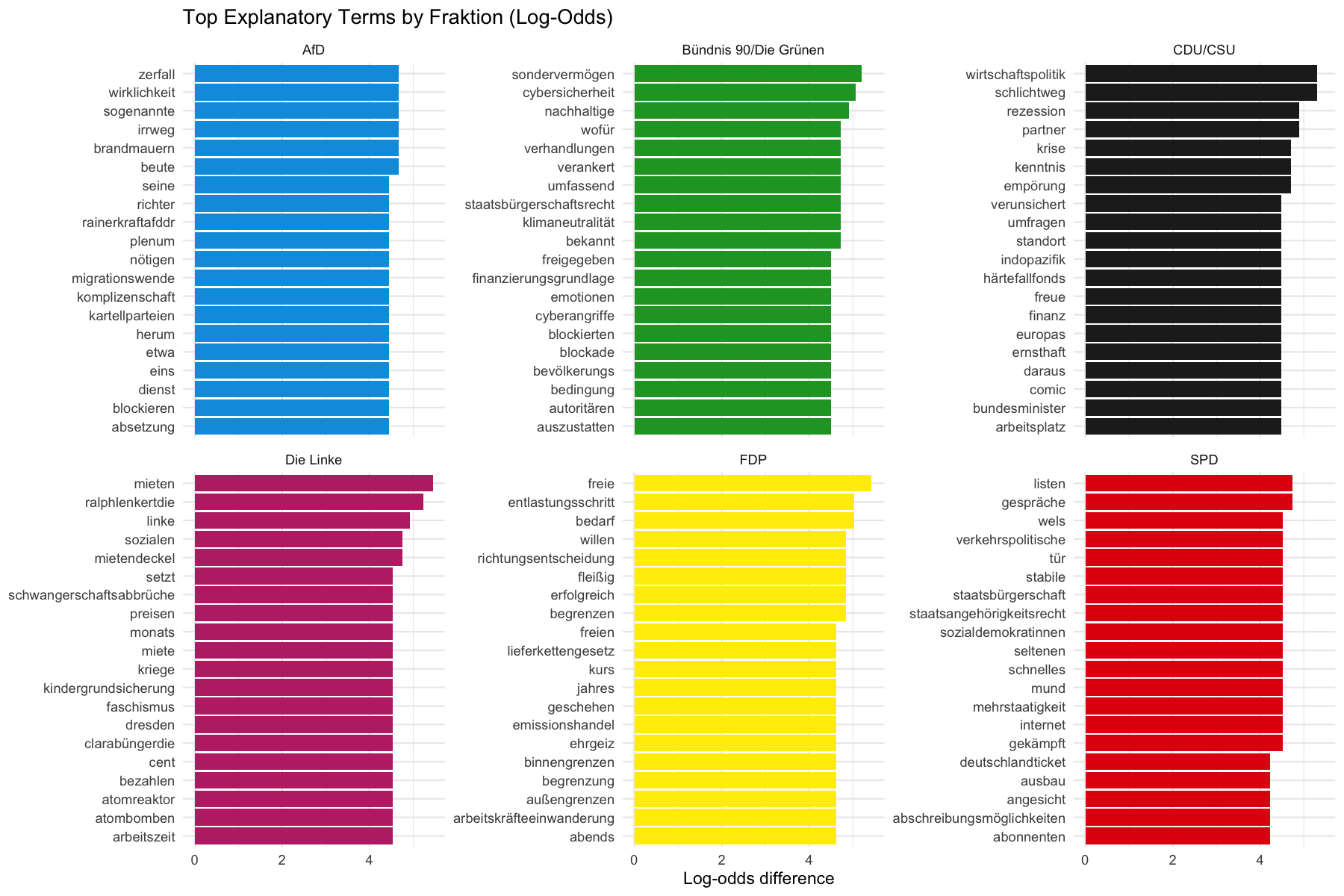
The bar charts in Figure 8 and Figure 9 are intentional: for comparison and reporting, they are generally more robust than pure word clouds.
Two patterns appear repeatedly:
- topical markers (policy-domain specific),
- rhetorical/debate markers (context-dependent).
For example, the global lists show terms like “Brandmauern” or “Grenzen” for AfD, “Klimaneutralität” and “Cybersicherheit” for the Greens, and “Mieten” and “Mietendeckel” for Die Linke. These are not hard rules, but taken together they form interpretable signals that align well with each party’s debate profile.
Hence, global top terms should always be read jointly with local chunk evidence: global terms show class patterns; local chunks provide instance-level rationale. In addition, speaker self-reference artifacts were explicitly filtered to avoid transcript-specific distortions.
Positioning and outlook
This study does not provide direct AI-Act risk classification. It does show that a transparent embedding-based setup can work reliably in a difficult multiclass setting when evaluation and model selection are done rigorously.
For me, the central message is: signal exists, but separation between semantically close classes is limited and must be operationally buffered through policy logic, thresholds, and review processes.
For real enterprise contexts, this is realistic. In governance-facing applications, a “perfect” classifier is rare; what matters is a robust end-to-end system of model, rules, monitoring, and traceable decision logic.
What we can take away
- Methodological feasibility: Embedding classification, conservative evaluation, and explainability can be combined into a reproducible pipeline.
- Evaluation discipline: Under class imbalance, Macro-F1 and Balanced Accuracy should be primary, not raw Accuracy alone.
- Operational pragmatism: A simple strong model (linear SVM) can be preferable in early product phases compared with maximum model complexity.
Limits
The main limits concern length, domain, and label semantics: Bundestag speeches are much longer than typical user prompts, and party labels are not equivalent to AI-Act risk labels. So this is not proof for the target task, but a controlled methodological stress test.
Still, the transfer logic is plausible: prompt-risk classes are also likely to be imbalanced, partially overlapping, and affected by asymmetric error costs. The current setup already captures these characteristics to a meaningful degree.
Next steps toward the target system
The next logical step is a domain-specific prompt dataset with a clear and documented AI-Act label scheme. On top of that, we need tiered decision design: class-specific thresholds, explicit escalation paths, and consistent human review for boundary cases.
Monitoring should be designed in from day one: drift in prompt distributions, class-wise error rates, recalibration, and version-safe audit logs are core requirements, not late add-ons.
Finally, evaluation should be extended with policy-facing KPIs, such as asymmetric error costs per risk class or latency constraints tied to service levels. That final mile determines whether a good offline model becomes a reliable control layer in live operation.
Reproducibility
The full data and modeling pipeline is available in the companion repository. This blog post loads pre-exported artifacts only and performs no API calls.
References
Bücker, Michael. 2026. “Bunddev: R Package for Working with German Bundestag and Related Parliamentary Data.” https://github.com/mchlbckr/bunddev.
Bücker, Michael, Gero Szepannek, Alicja Gosiewska, and Przemyslaw Biecek. 2021. “Transparency, Auditability, and Explainability of Machine Learning Models in Credit Scoring.” Journal of the Operational Research Society 73 (1): 70–90. https://doi.org/10.1080/01605682.2021.1922098.
Cortes, Corinna, and Vladimir Vapnik. 1995. “Support-Vector Networks.” Machine Learning 20 (3): 273–97. https://doi.org/10.1007/BF00994018.
Doshi-Velez, Finale, and Been Kim. 2017. “Towards a Rigorous Science of Interpretable Machine Learning.” arXiv Preprint arXiv:1702.08608. https://arxiv.org/abs/1702.08608.
European Union. 2024. “Regulation (EU) 2024/1689 Laying down Harmonised Rules on Artificial Intelligence (AI Act).” https://eur-lex.europa.eu/eli/reg/2024/1689/oj.
Federal Returning Officer of Germany. 2021. “Election to the 20th German Bundestag on 26 September 2021: Final Result by Constituencies.” https://www.bundeswahlleiterin.de/en/bundestagswahlen/2021/ergebnisse/bund-99.html.
Lundberg, Scott M., and Su-In Lee. 2017. “A Unified Approach to Interpreting Model Predictions.” In Advances in Neural Information Processing Systems 30. https://proceedings.neurips.cc/paper/2017/hash/8a20a8621978632d76c43dfd28b67767-Abstract.html.
Ribeiro, Marco Tulio, Sameer Singh, and Carlos Guestrin. 2016. “Ẅhy Should i Trust You?:̈ Explaining the Predictions of Any Classifier.” In Proceedings of the 22nd ACM SIGKDD International Conference on Knowledge Discovery and Data Mining, 1135–44. https://doi.org/10.1145/2939672.2939778.
Vapnik, Vladimir N., and Alexey Y. Chervonenkis. 1971. “On the Uniform Convergence of Relative Frequencies of Events to Their Probabilities.” Theory of Probability & Its Applications 16 (2): 264–80. https://doi.org/10.1137/1116025.